Most churn models fail for one simple reason: they look at a customer’s status, not the change that happened before churn. If I want earlier churn warnings, I need point-in-time features built from behavior over time, not one static snapshot.
Here’s the short version:
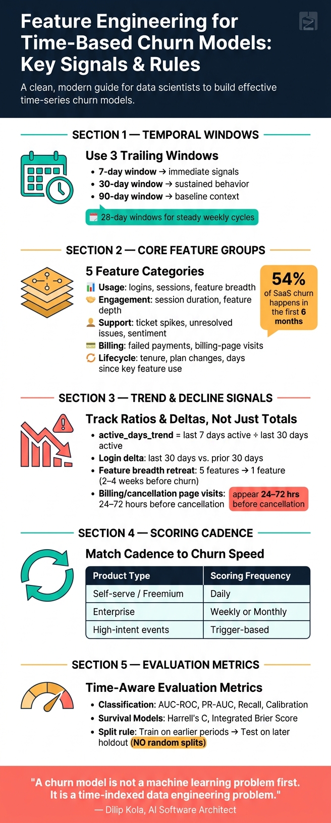
- I should use time-based windows like 7, 30, and 90 days
- I should focus on decline signals, such as drops in logins, usage, spend, or feature breadth
- I need a fixed observation date so every feature only uses past data
- I should avoid data leakage and use calendar-based train/validation/test splits
- I can build for classification or survival analysis, depending on whether I care more about if churn happens or when
- I should score on a set cadence: daily for fast-moving self-serve products, weekly or monthly for slower enterprise cycles
- I need features from usage, support, billing, tenure, and plan history
- I should track trend features like ratios, deltas, and velocity, not just totals
- I should tie model output to revenue, such as "$47,000 in MRR at risk", not just account counts
- I need time-aware evaluation with metrics like PR-AUC, recall, calibration, and for survival models Harrell’s C and Integrated Brier Score
A few facts stand out. In some SaaS data, 54% of churn happens in the first 6 months. And behavior shifts like billing-page visits or sudden usage drops can show up 24–72 hours before cancellation. That means timing rules, window design, and feature freshness matter as much as the model itself.
If I had to sum up the article in one line, it would be this: a churn model works best when I turn each customer history into clean, dated snapshots that show slowdown, friction, and intent before the customer leaves.
Key Feature Groups & Signals for Time-Based Churn Models
Core Temporal Feature Groups for Churn Models
Start with windowed usage, then add signals that show strain and slowdown.
Recency, Frequency, and Monetary Features Across Trailing Windows
Recency, Frequency, and Monetary (RFM) features are the backbone of most churn models. Recency tracks the days since a customer last logged in, made a purchase, or submitted a payment. Frequency counts things like sessions, orders, or product actions. Monetary measures billed revenue, plan value, upgrades, and downgrades.
Use 7-, 30-, and 90-day trailing windows from the same cutoff point. That setup helps you see whether activity is picking up or fading before churn happens. For example, a user who logged in 15 times over 30 days but only once in the last 7 days can still look active in a monthly report. But the short-term pattern tells a different story: momentum has slowed in a clear way.
From there, add engagement, support, payment, and lifecycle signals.
Engagement, Support, Payment, and Lifecycle Timeline Features
Raw usage counts only tell part of the story. A second layer of features helps show account health in more detail. This can include session frequency, feature breadth, session duration, days since first use of a key feature, and days since the last plan change. Tenure also matters a lot. Risk is often highest in the first 3 to 6 months, then drops as the account gets older. In some SaaS datasets, about 54% of churn happens within the first 6 months.
Support and billing signals can sharpen the picture. A spike in support tickets, unresolved issues, or negative-sentiment messages often points to friction before a customer even starts thinking about canceling. Failed payments and visits to billing or cancellation pages are strong intent signals, and they often call for immediate intervention. In many cases, those signs show up before the customer makes the final decision to leave.
Churn often starts as visible friction long before cancellation.
Then measure decline with ratios and deltas, not raw counts alone.
Trend and Change Features That Detect Decline
Static features show what a customer is. Trend features show what the customer is becoming. That distinction matters. The gap between a customer's last 30 days and the prior 30 days - in logins, feature usage, or spend - is often more predictive than either window by itself. Churn usually looks less like a cliff and more like a slow fade.
One useful example is active_days_trend, defined as the ratio of active days in the last 7 days to active days in the last 30 days. In one 2026 LightGBM churn study across 8,400 customers, it ranked among the strongest predictors. Ratios like that can reveal a drop in pace that raw totals may hide. It also helps to track narrowing feature use. When a customer goes from using five product features to one, that retreat often comes 2 to 4 weeks before cancellation.
Churn models need usage, engagement velocity, and support signals - not logins alone.
sbb-itb-17e8ec9
Designing Windows, Cadence, and Labels
After you define the features, the next job is to lock down the time rules that make those features usable in production.
Choose Window Lengths Based on the Prediction Horizon
Use short, medium, and long windows together. That mix helps you pick up immediate signals, sustained behavior, and baseline context.
If you're predicting 30-day churn, pair a 7-day short window with a 90-day baseline. The short window picks up what's happening now. The long window gives you the context to tell whether that signal is unusual, which matters for early detection.
Use 28-day windows when you need steady weekly cycles.
Set a Scoring Cadence and Rebuild Features on a Fixed Schedule
Keep scoring on a fixed schedule so features, labels, and monitoring stay in sync. Rebuild features on a fixed schedule that matches how fast customers can churn and how fast teams can respond.
Match cadence to the speed of churn. Self-serve or freemium products tend to do best with daily scoring, while enterprise accounts can often work with weekly or monthly refreshes. Add trigger-based scoring for high-intent events.
Scoring frequency decides when you act. Label design decides what the model learns.
Define Churn Labels for Classification and Survival Setups
For classification, label churn inside the prediction window after the observation date. The observation date is a hard cutoff: features come from before it, and labels come from after it.
For survival analysis, record time to churn and mark customers who have not churned by the end of the study as censored - meaning churn has not occurred by the study end.
Use a 7–30 day buffer between observation and outcome so the team has time to act.
With windows, cadence, and labels fixed, the next step is building a pipeline that can produce them in a steady, repeatable way.
Building Temporal Feature Pipelines That Work in Production
Once windows, labels, and cadence are set, the next step is to turn them into repeatable point-in-time snapshots.
Structure Source Data Around Customers, Events, Payments, and Support
In production, churn pipelines turn those temporal features into snapshots tied to a specific observation date. Most teams pull from customer, event, billing, and support tables that hold plan data, usage data, payment records, and support tickets.
The core rule is as-of-date correctness. Every join and aggregate should be filtered by the observation date so no future record slips into the feature set. A simple way to enforce that is to store one row per customer per snapshot date. With that setup, you can audit exactly what the model could have seen on any given date.
Compute Features in Batch or Real Time Based on Business Needs
For most teams, batch computation in a SQL warehouse is the right place to start. An Airflow DAG that scores customers and pushes high-risk flags into the CRM handles the bulk of churn use cases.
Say you need a billing feature. You might count failed payments in the prior 90 days. You'd also want to store repeat windowed aggregates - like 30-day login counts, 90-day payment failure rates, and trend ratios - in dbt models or warehouse tables. That keeps scoring fast and keeps runs consistent over time.
Real time only makes sense when the model has to react before the next batch run. For freemium or self-serve products, abrupt behavior shifts - like visits to the billing page or a drop in sessions - can show up 24–72 hours before cancellation. In that kind of setup, a streaming layer like Kafka or RisingWave, paired with an online store like Redis, lets you score users and trigger outreach within minutes.
A practical split looks like this:
- Use batch for stable account metadata
- Use near real time for engagement trends
- Use streaming only for fast behavioral shocks
Connect Churn Features to Startup Forecasting and Reporting
Churn scores get much more useful when you translate them into revenue. Instead of saying "320 accounts at risk," say "$47,000 in MRR at critical risk" by multiplying each customer's churn probability by expected future margin. That's the kind of number finance teams and board members can act on.
Those scores should feed straight into revenue forecasts and retention scenarios so finance and growth teams work from the same numbers. From there, the outputs need to be checked with time-aware validation and drift monitoring.
Evaluating and Refining Temporal Features Over Time
Measure Model Quality with Time-Aware Evaluation
Once the feature pipeline is stable, test it under the same time rules it will face in production. That means no random train/test split. Train on earlier time periods, test on a later holdout, and make sure every feature stays point-in-time correct.
Then look at metrics that match the job. Overall accuracy can look fine while the model still misses the cases you care about. For classification, use AUC-ROC, PR-AUC, recall, and calibration. If churn is rare, PR-AUC and calibration deserve extra attention. For survival models, use Harrell's C to rank churn timing and the Integrated Brier Score to check probability calibration across the full time horizon.
Interpret Feature Impact and Monitor Drift
A model score only helps if the retention team can do something with it. Use SHAP with tree-based models to show what pushed the score up or down, whether that was lower engagement, failed payments, or support friction. A customer flagged because of an 80% drop in engagement velocity needs a different response than someone flagged for repeated failed payments.
Behavior also changes over calendar time. That's a temporal issue, not just routine upkeep. Track weekly score shifts, then retrain monthly on the latest six months only if the new model beats the current one on a held-out future period.
Conclusion: The Temporal Features That Matter Most
Use these checks to keep the model reliable as behavior changes over time.
"A churn model is not a machine learning problem first. It is a time-indexed data engineering problem." - Dilip Kola, AI Software Architect
FAQs
How do I choose the right time windows for my churn model?
Define your observation and prediction windows around how customers usually behave, not random calendar cutoffs.
The observation window is the past period you use to build features. The prediction window is the future period you want to forecast.
It also helps to add a buffer window between the two. That gap reduces reactive signals and gives you a cleaner setup.
For trend data, use rolling aggregates like:
- 7-day
- 30-day
- 90-day
One more thing: always calculate features from a fixed snapshot date. That helps prevent data leakage and keeps your training setup aligned with production logic.
When should I use classification instead of survival analysis?
Use classification when you want to estimate the chance of churn or assign a probability score based on customer behavior. It works best when you're linking static snapshots, like current demographics or plan attributes, to a binary churn outcome.
Pick it when time-based behavior can be boiled down into a fixed set of independent features, such as RFM metrics. If your main goal is to predict when churn will happen, use survival analysis instead.
What are the most common causes of data leakage in churn features?
Data leakage happens when churn features use information that wouldn’t exist yet at the moment you make the prediction.
That’s the core issue: the model ends up learning from the future. And when that happens, results can look far better than they’d be in production.
Common causes include:
- look-ahead windows in rolling metrics or averages
- joining status or payment fields updated after the prediction point
- using
now()instead of a row timestamp - missing exact cutoff times in SQL joins
- random train-test splits that let future data leak into training